11. ReLU and Softmax Activation Functions
Activation functions
Previously, we've been using the sigmoid function as the activation function on our hidden units and, in the case of classification, on the output unit. However, this is not the only activation function you can use and actually has some drawbacks.
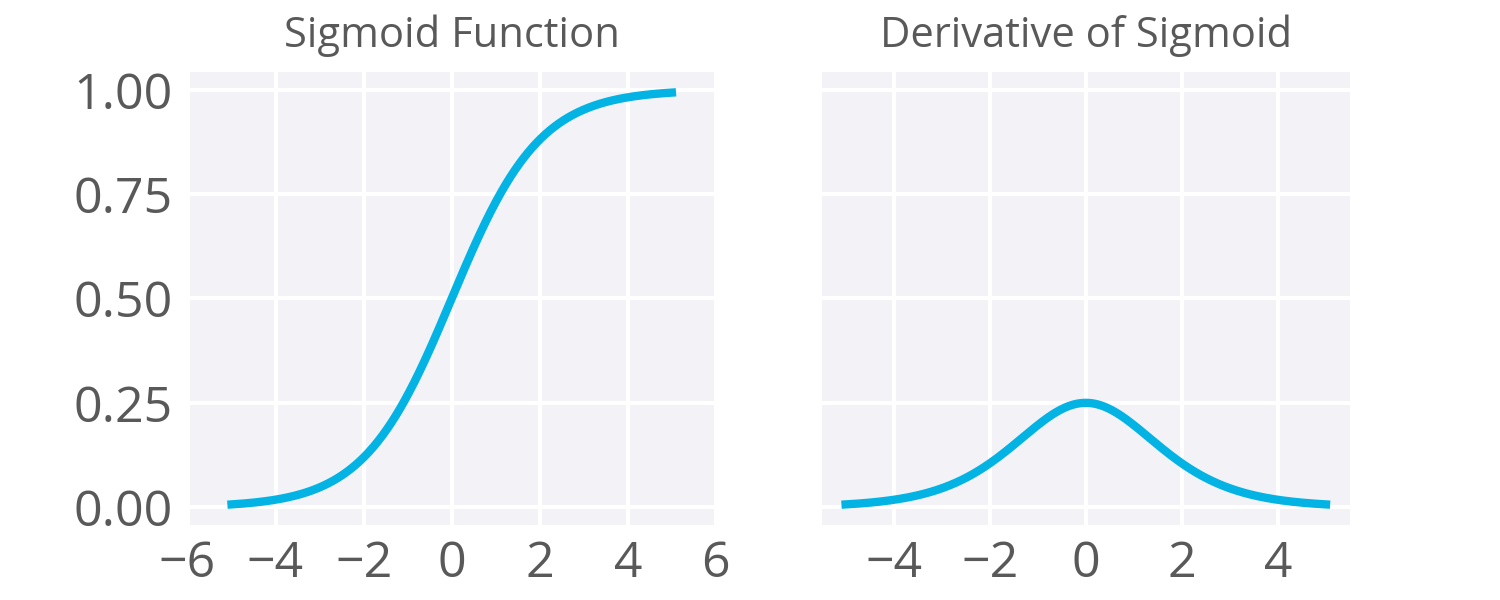
As noted in the backpropagation material, the derivative of the sigmoid maxes out at 0.25 (see above). This means when you're performing backpropagation with sigmoid units, the errors going back into the network will be shrunk by at least 75% at every layer. For layers close to the input layer, the weight updates will be tiny if you have a lot of layers and those weights will take a really long time to train. Due to this, sigmoids have fallen out of favor as activations on hidden units.
Enter Rectified Linear Units
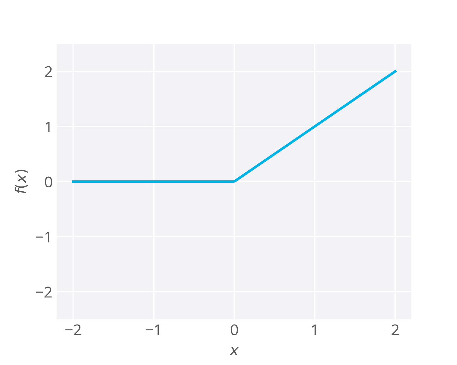
Instead of sigmoids, most recent deep learning networks use rectified linear units (ReLUs) for the hidden layers. A rectified linear unit has output 0 if the input is less than 0, and raw output otherwise. That is, if the input is greater than 0, the output is equal to the input. Mathematically, that looks like
f(x) = \mathrm{max}(x, 0).
The output of the function is either the input, x , or 0 , whichever is larger. So if x = -1 , then f(x) = 0 and if x =0.5 , then f(x) = 0.5 . Graphically, it looks like:
ReLU activations are the simplest non-linear activation function you can use. When the input is positive, the derivative is 1, so there isn't the vanishing effect you see on backpropagated errors from sigmoids. Research has shown that ReLUs result in much faster training for large networks. Most frameworks like TensorFlow and TFLearn make it simple to use ReLUs on the the hidden layers, so you won't need to implement them yourself.
Drawbacks
It's possible that a large gradient can set the weights such that a ReLU unit will always be 0. These "dead" units will always be 0 and a lot of computation will be wasted in training.
From Andrej Karpathy's CS231n course:
Unfortunately, ReLU units can be fragile during training and can “die”. For example, a large gradient flowing through a ReLU neuron could cause the weights to update in such a way that the neuron will never activate on any datapoint again. If this happens, then the gradient flowing through the unit will forever be zero from that point on. That is, the ReLU units can irreversibly die during training since they can get knocked off the data manifold. For example, you may find that as much as 40% of your network can be “dead” (i.e. neurons that never activate across the entire training dataset) if the learning rate is set too high. With a proper setting of the learning rate this is less frequently an issue.
Softmax
Previously we've seen neural networks used for regression (bike riders) and binary classification (graduate school admissions). Often you'll find you want to predict if some input belongs to one of many classes. This is a classification problem, but a sigmoid is no longer the best choice. Instead, we use the softmax function. The softmax function squashes the outputs of each unit to be between 0 and 1, just like a sigmoid. It also divides each output such that the total sum of the outputs is equal to 1. The output of the softmax function is equivalent to a categorical probability distribution, it tells you the probability that any of the classes are true.
The only real difference between this and a normal sigmoid is that the softmax normalizes the outputs so that they sum to one. In both cases you can put in a vector and get out a vector where the outputs are a vector of the same size, but all the values are squashed between 0 and 1. You would use a sigmoid with one output unit for binary classification. But if you’re doing multinomial classification, you’d want to use multiple output units (one for each class) and the softmax activation on the output.
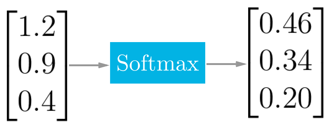
For example if you have three inputs to a softmax function, say for a network with three output units, it'd look like:
Mathematically the softmax function is shown below, where \mathbf{z} is a vector of the inputs to the output layer (if you have 10 output units, then there are 10 elements in \mathbf{z}). And again, j indexes the output units.
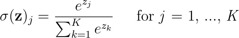
This admittedly looks daunting to understand, but it's actually quite simple and it's fine if you don't get the math. Just remember that the outputs are squashed and they sum to one.
To understand this better, think about training a network to recognize and classify handwritten digits from images. The network would have ten output units, one for each digit 0 to 9. Then if you fed it an image of a number 4 (see below), the output unit corresponding to the digit 4 would be activated.
Image from the MNIST dataset
Building a network like this requires 10 output units, one for each digit. Each training image is labeled with the true digit and the goal of the network is to predict the correct label. So, if the input is an image of the digit 4, the output unit corresponding to 4 would be activated, and so on for the rest of the units.
For the example image above, the output of the softmax function might look like:
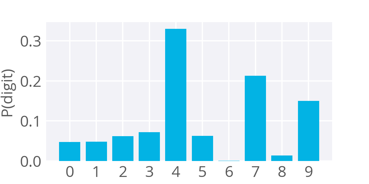
Example softmax output for a network predicting the digit shown above
The image looks the most like the digit 4, so you get a lot of probability there. However, this digit also looks somewhat like a 7 and a little bit like a 9 without the loop completed. So, you get the most probability that it's a 4, but also some probability that it's a 7 or a 9.
The softmax can be used for any number of classes. As you'll see next, it will be used to predict two classes of sentiment, positive or negative. It's also used for hundreds and thousands of classes, for example in object recognition problems where there are hundreds of different possible objects.